2 Density-independent growth
Learning Objectives
From this lesson, you will be able to…
- Identify the key features of exponential and geometric population growth.
- Explain how and when exponential and geometric growth are relevant biologically, including the initial spread of an infectious disease.
- Understand the difference between per capita growth rate and population growth rate.
- Articulate the difference between “net reproductive growth” (\(R_0\)) and intrinsic growth rate (\(r\)).
- Explain how birth rate, death rate, and juvenile growth/maturation rate combine to shape overall population growth.
2.1 Introduction
Let’s start with a question:
Question 1: In a pond, there is a patch of lily pads. Each day, the patch doubles in size (i.e., the number of lily pads doubles). If it takes 48 days for the patch to cover the entire lake, how long would it take for the patch to cover half of the lake? ____ days.
Answer:
2.1.1 Explanation
If you got the question right, congrats!
If you got it wrong, don’t feel bad! Many students at elite universities got it wrong as well (Frederick, 2005).
\(\qquad\) If you got it wrong, I suspect you thought the answer was \(24\). After all, it seems reasonable that it would take half the total number of days (\(24/48 = 1/2\)) to fill half the pond. This would be the case if the lily pad patch grew linearly (Figure 1A). Under linear growth, the lily pad population would grow by a constant amount over each time interval and would indeed be half-full after \(24\) days.
\(\qquad\) However, the number of lily pads doubles every day. It does not grow linearly (Figure 1B) — the number of lilies doubles each time step. This is a form of exponential growth (technically, it is geometric growth — these are very similar terms that we will distinguish later).
\(\qquad\) This is easiest to see with a cartoon depicting the lily pads in the pond over time:
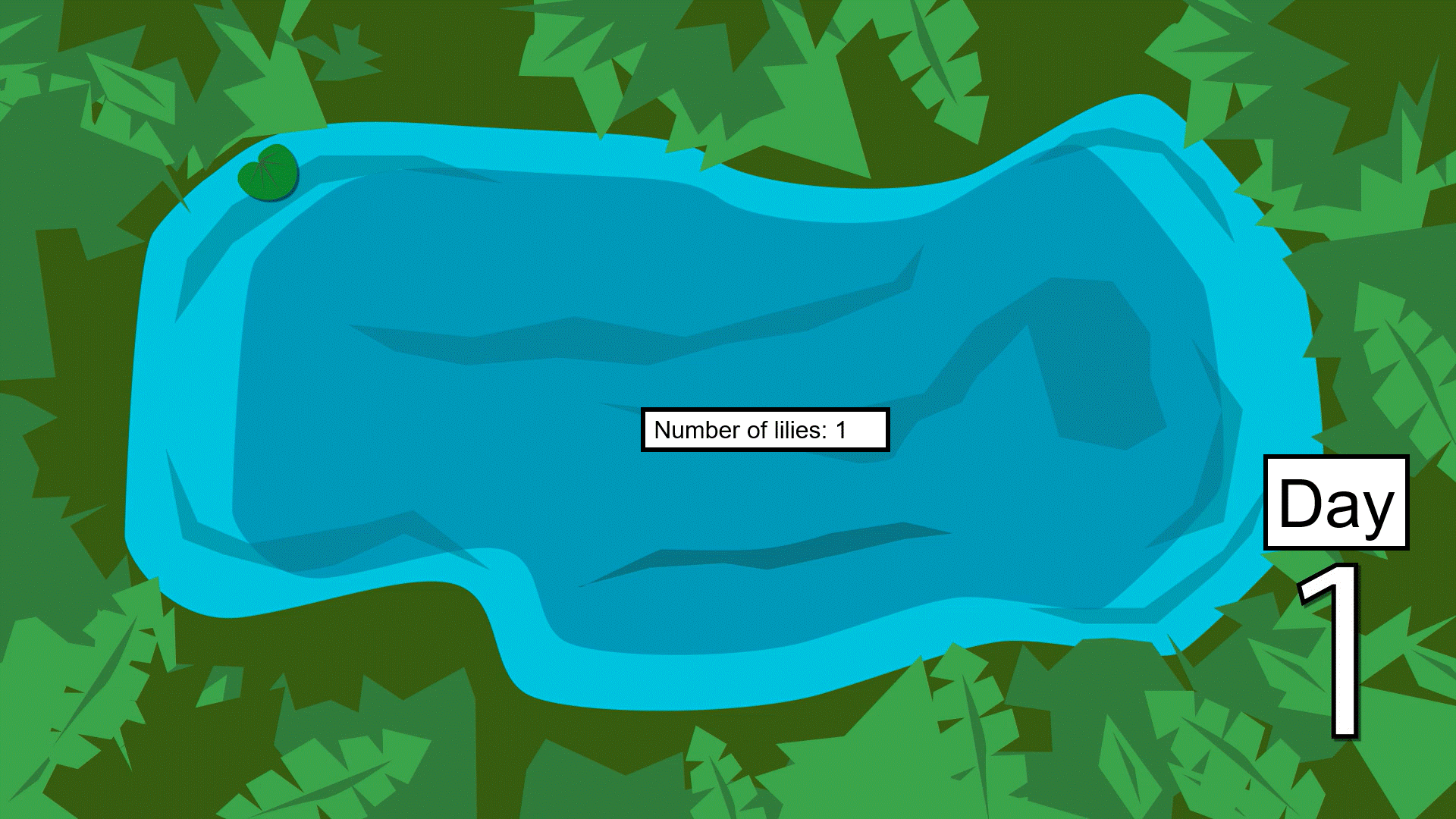
The number of new lilies that appear each day is not constant because the lily pads double in number each day. In other words, their increase each day is proportional to how many there are. If there were \(128\) lily pads on a given day, it means there were \(64\) the previous day (an increase of \(64\) lilies). The day before there were \(64\) lilies, there were \(32\) (an increase of \(32\) lilies). \(64 \neq 32\), and thus the total number of lily pads increases non-linearly.
\(\qquad\) The pond is not halfway full until the second-to-last day. If it takes \(48\) days to fill the pond (as in the initial question), it will be half full on day \(47\) (the correct answer). Half of all the lily pads found in the pond on a given day always appeared on that day.
Question 2: If the pond were to take D days to fill with doubling lily pads (the same scenario as before), the pond will be \(1/4\) full on day _____. Fill in the blank in terms of D.
Answer:
\(\qquad\) Why do many people get this question wrong? The confusion reflects the fact that the patch of lily pads is growing exponentially and exponential growth is simply not intuitive. When posed with the question, many people substitute the more “intuitive-but-incorrect” linear growth (Figure 2.1A). If something is growing exponentially, not much seems to happen initially – and then suddenly, it explodes (Figure 2.1B). Due to this property, it is easy to underestimate just how rapidly something can change in size, abundance, or prominence if it grows exponentially.
The counter-intuitive nature of exponential growth leads to some amusing thought experiments. Imagine folding a piece of paper in half repeatedly. Initially, the thickness increases slowly. However, by the 10th fold, it would be the width of your hand. By the 20th fold (which isn’t even close to physically possible, but bear with me), it could reach the height of a building.
2.1.2 Why should I care?
With some consideration, the above discussion can give us insights into the following questions:
\(\qquad \qquad\) Why did we feel the need to perform lockdowns during the COVID-19 pandemic?
\(\qquad \qquad\) What do we fear when an “exotic” species is introduced to an ecosystem?
Many of our worries can be summarized by the simple yet powerful phenomenon of exponential growth (or geometric growth, which is nearly the same thing). Geometric and exponential growth refer to when a population grows unbounded, increasing at a rate proportional to its population size. In other words, the population increases by a constant proportion each interval of time (e.g., doubling in size every day, as in the lily pad example). A population that is initially small can rapidly increase in abundance/number if it grows exponentially. In the case of COVID-19, we were concerned that a small number of cases would balloon into millions (which indeed happened).
\(\qquad\) We often call exponential/geometric growth “density-independent” growth. This is because, in nature, we realistically expect population growth rates to change with population size/density. Typically, we expect the population growth rate to decrease with population size/density eventually because a population cannot grow forever. Density-dependent factors, such as limited resources (or limited hosts to infect, if you’re a disease like COIVD-19), eventually slow down and limit population growth, preventing it from continuing indefinitely. However, population growth may be initially exponential/geometric.
Question 3: How does exponential growth differ from linear growth?
Answer: In linear growth, the quantity (e.g., the number of lily pads) increases by a constant amount over a fixed interval of time. For exponential growth, the quantity (e.g., the number of lily pads) increases by a constant proportion over a fixed interval of time. See Figure 2.1A vs. 2.1B for a visualization.
Something along these lines is correct — you may phrase it differently. The key is to make sure you understand the difference between increasing by a fixed amount vs. a fixed proportion. When something increases by a fixed amount, the magnitude of the increase does not depend on how much of it there is (e.g., the increase in lily pads would not depend on how many there are). However, if something increases by a fixed proportion, the magnitude of the increase very much depends on how much of it there is. This is the crucial distinction.
With this in mind, let’s explore exponential / geometric growth. The first thing to get an intuition about what exponential growth looks like:
What does exponential growth look like?
Before we dive into the math of exponential (and geometric) growth, it’s helpful to get an intuition about what it “looks” like. Exponential population growth has a distinctive “shape.” By shape, I mean how population size/abundance/density \(N(t)\) increases over time.
\(\qquad\) Below are three examples: (1) the initial waves of COVID-19 infections, (2) invasive Monk Parakeets, and (3) a recovering population of bison. Population growth may be initially exponential/geometric.
\(\qquad\) The initial waves of COVID-19 infections grew exponentially across the globe (e.g., France in Figure 2.3A). Here, the “population” of interest is the number of infected people.
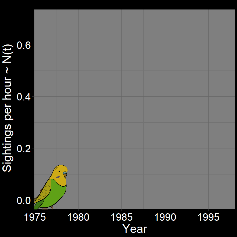
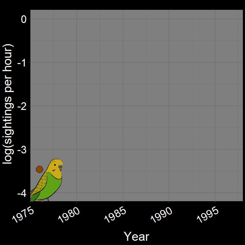
\(\qquad\) Monk Parakeets (while cute) are an invasive species in the United States (among other countries). Like COVID-19, Monk Parakeets exhibited exponential growth for a number of years (Figure 2.3B). Notice that bird observations were made during Christmas Bird Counts, hence the unusual unit of “Sightings per hour ~ \(N(t)\)” on the \(y\)-axis. The original study (Val Basel and Pruett-Jones, 1996) used the bird counts as a proxy for population size.
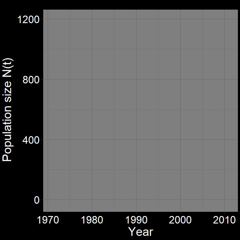
\(\qquad\) Exponential growth can also be a “good” thing: after facing near extinction, bison populations in the USA have exhibited years of exponential population growth, in part due to conservation efforts (Figure 2.3C). These data imply that the bison population is recovering exponentially, at least for now.
\(\qquad\) Exponential growth can be both beneficial and harmful, depending on the context. Rapid growth in invasive species or infectious diseases can lead to significant ecological and health challenges. Conversely, exponential growth in endangered species populations can signal successful conservation efforts and ecological recovery.
So, what causes growth to look like these three examples? Why do populations (at least initially) tend to grow like this? Why are exponential and geometric growth such “natural” ways to think about growth?
2.2 Geometric growth and exponential growth models
Below, we’ll explore the logic behind geometric and exponential growth models. My goal is for you to understand why these forms of growth are, arguably, the simplest assumptions one might make about population growth.
\(\qquad\) We will start with geometric growth, then discuss exponential growth and how they differ.
2.2.1 Geometric growth per se
There are different philosophies for building a population model, even when they are simple. Let’s think about population change. In our introduction, we talked about how to construct a model.
\(\qquad\) We might think about constructing a model with this structure in mind:
\[ \underbrace{N(t + 1)}_{\text{Abundance at next time step}} = \underbrace{N(t)}_{\text{Abundance at previous step}} \; \; + \; \; \text{increase} \; \; - \; \; \text{decrease} \tag{2.1}\]
where \(N(t)\) is the population abundance at time \(t\), and \(N(t + 1)\) is the abundance after one unit of time. In practice, the unit of time might be how often one measures the abundance of a population. The terms “increase” and “decrease” represent how much the population increases and decreases each time unit — our goal here is to fill these in. In this first attempt, let’s assume the “increase” and “decrease” terms only reflect births and deaths (i.e., there is no immigration of individuals in or emigration of individuals out of the population; see “Course Introduction”).
\(\qquad\) To make things more concrete, let’s assume we’re talking about a plant population that we observe each year \(t\). Each year (thus the \(+1\) in \(t+1\) is one year), plants produce seeds that turn into reproductive plants (the “increase”). In addition, each year, some proportion of plants die after producing seeds. Furthermore, we assume all individuals in the population reproduce (so, we are either ignoring males, or we assume the population reproduces asexually).
\(\qquad\) Below is a video that shows this over a single time step, from \(t\) to \(t+1\):
Above, we defined geometric growth as “when a population grows unbounded, increasing at a rate proportional to its population size.” What would that mean for our plant model? Instead of trying to “get to” geometric growth (as if it’s some kind of goal), it is much better scientific practice to ask ourselves the question, “What are the simplest assumptions we could make to model population growth?”
Question 4 Take a moment and ask yourself the question: “How might I model births and deaths for our plant model in a way that is biologically feasible, but very simple?” (The point of this question is to get you thinking about making a model, not necessarily to get the “correct” answer).
Think about the meaning of the term “density-independent” (as defined above) and apply that to the “increase” and “decrease” terms. Additionally, consider the model unfolding in terms of “what happens to each individual / what each individual does” instead of “how does the population change?”
Each individual in the population just “does its thing”.
- Each reproductive plant in the population gives birth to a fixed number of seeds each time step
- Each reproductive plant has a fixed chance of dying each year
Therefore, the number of births of each individual and the probability each individual dies does not depend on the number of individuals in the population (emphasizing the density-independent aspect).
As it turns out, these assumptions this will give us geometric growth.
With the above idea in mind, let’s tackle births. We are assuming that each individual in the population gives birth to a fixed number of seeds each time step. We might assume that, each time step, the first thing each individual does is give birth to \(\text{b}\) individuals.
Question 5A: with this assumption in mind, \(\text{increase}=\) ___ ?
\[ \text{increase} = \text{b} N(t) \tag{2.2}\]
Each plant gives birth to \(\text{b}\) new individuals, so the total number of births is \(\text{b}\) multiplied by the number of individuals \(N(t)\).
This leads to a very important concept. The total increase of the population is \(\text{b} N(t)\). However, each plant produces \(\text{b}\) offspring (seeds). We call this the per capita births (essentially, births per individual).
Question 5B: what range of values might \(\text{b}\) take?
Strictly speaking, we assuming
\[ 0 \leq b < \infty \] That is, each plant can produce any number of seeds, and a plant cannot produce a negative number of seeds.
\(\qquad\) Similarly, our principle is that a fixed portion of reproductive plants \(\text{d}\) die each time step after producing seeds. A more biological way to think about this is that, on average, each reproductive plant has a probability of death \(\text{d}\).
Question 6A: with the above in mind, \(\text{decrease}=\) ___ ?
\[ \text{decrease} = \text{d} \times N(t) \]
Similar to the birth case, \(\text{d}\) is per capita mortality.
\(\qquad\) One way to think about this is that the average probability an individual dies is \(\text{d}\). That is, on a given timestep of the model, if I were to randomly pick a reproductive adult, the probability that it dies is equal to \(\text{d}\).
Question 6B: what range of values might \(\text{d}\) take?
\(\leq \text{d} \leq\)
\(\text{d}\) is a proportion/probability, so can only takes values between 0 and 1.
\(\qquad\) These questions emphasize an absolutely crucial concept – per capita births and deaths. While it is natural to think about what the overall population does, it is often best (and easier) to think about what individuals do. Typically, we think of (e.g.) per capita births and deaths as what the average individual does. By thinking about “what does an individual do?”, we can build models from the ground up, where the collective individual changes shape the population dynamics (and not the other way around).
From this, we can construct our model.
Question 7A: Substitute the values of “increase” and “decrease” into equation (\(2.1\)) for our plant model.
\[ \underbrace{N(t + 1)}_{\text{Abundance at year } t + 1} = \underbrace{\text{b} N(t)}_{\text{total births}} + \underbrace{\big(1-\text{d}\big)N(t)}_{\text{proportion that die}} \tag{2.3}\] or, we might write it as: \[ N(t + 1) = N(t)\big(1 + \text{b} - \text{d}\big) \tag{2.4}\]
Question 7B: By what proportion does our population change each time step (e.g. each year in our plant model)?
From \[ N(t + 1) = \big(1 + \text{b} - \text{d}\big) N(t) \] we can write \[ \frac{N(t + 1)}{N(t)} = 1 + \text{b} - \text{d} \] Hence, the yearly proportional change is \(1 + \text{b} - \text{d}\). We typically label this as \(\lambda\) and call it the “finite rate of increase”: \[ \lambda = 1 + \text{b} - \text{d} \tag{2.5}\]
So, we can also rewrite Equation 2.4 as
\[ N(t + 1) = \lambda N(t) \]
Using our rewriting from equation with Equation 2.5, we have
\[ N(t + 1) = \lambda N(t) \tag{2.6}\]
where the proportional increase each timestep is \(\lambda\):
\[ \frac{N(t + 1)}{N(t)} = \lambda \tag{2.7}\]
So, if we know the abundance \(N(t)\) and we know \(\lambda\), we can find \(N(t+1)\). However, We don’t just want to know what happens between time \(t\) and \(t+1\). Rather, we want to know, “If we know the abundance at time \(0\), what will the abundance be at time \(t\)?” We can calculate this too:
Deriving the trajectory of geometric growth
Question 8A: Let us start with population abundance \(N(0)\) (that is, \(t=0\)). \(N(0)\) can be any positive abundance greater than zero (there is at least one individual in the population). What will the population abundance be at time \(t=1\)?
We know \[ N(t+1) = \lambda N(t) \] so, \[ N(1) = \lambda N(0) \]
Question 8B: Let us start with population abundance \(N(0)\) (that is, \(t=0\)). What will the population abundance be at time \(t=2\)?
We know \[ N(1) = N(0)\lambda \] so, \[ N(2) = \lambda N(1) \] We can then substitute \(N(1) = \lambda N(0)\) to get
\[\begin{split} N(2) &= \lambda N(1) \\ & = \lambda \times \big[\lambda N(0)\big]\\ & = \lambda^2 N(0) \end{split}\]Question 8C: Again starting at population abundance \(N(0)\), what will the population abundance be at time \(t\)? Apply the logic from the above question.
\[ N(t) = \lambda^t N(0) \tag{2.8}\]
So, we now have our geometric growth model! Let’s make sure we understand its key properties.
Population increase and decrease for geometric growth
It is essential that you understand whether a population increases or decreases. This is simple, but fundamental:
Question 9A: Express the condition under which the population increases in terms of λ.
\(\lambda >\)
Question 9B: Express the condition under which the population decreases in terms of λ.
\(\lambda <\)
Question 9C: Express when the population will increase in terms of b and d:
\(>\)
Question 9D: Rewrite the above in terms of b/d. That is, the population will increase when:
\(\frac{\text{b}}{\text{d}} >\)
Try it yourself!
Please play around with this Shiny interactive web app, Module 2.1. In the module, you can examine the population trajectory of the model for different values of \(\text{b}\) and \(\text{d}\). Notice what happens when e.g. \(\text{b}/\text{d}<1\).
I find the condition from Question 9D (\(\text{b}/\text{d}>1\)) to be particularly intuitive. The intuitive nature of the \(\text{b}/\text{d}>1\) condition becomes clearer if you recognize that \(1/\text{d}\) is the average number of years a plant lives (see an explanation for this below below).
Question 10A: Given that \(\frac{1}{\text{d}}\) is the average number of years a plant lives, interpret \(\frac{\text{b}}{\text{d}}\).
Answer: \(\frac{\text{b}}{\text{d}}\) can be interpreted as “the average number of new plants (offspring) a plant produces over its lifetime.”
\(\text{b}\) is the average number of offspring (seeds) a plant produces per year. If we recognize that \(1/\text{d}\) is the average number of years a plant lives, then \(\frac{\text{b}}{\text{d}}\) can be seen as:
\[\begin{split} \frac{\text{b}}{\text{d}} & = \text{b} \times \frac{1}{\text{d}} \\ & = \bigg(\frac{\text{b births}}{\cancel{\text{year}}}\bigg) \times \bigg(\frac{1}{\text{d}} \frac{\cancel{\text{years}}}{\text{lifetime}} \bigg) \\ & = \frac{\text{b}}{\text{d}} \frac{\text{births}}{\text{lifetime}} \end{split}\]Therefore, \(\frac{\text{b}}{\text{d}}\) is the average number of births (offspring) it produces per lifetime.
Question 10B: Why should \(\frac{\text{b}}{\text{d}}>1\) indicate population growth?
Answer: Each plant is (obviously) a single individual. When it dies, \(N(t)\) decreases by one individual. Therefore, for the population to grow, the average plant must more than just replaces it self – that is, over its lifetime, the average plant must produce more than one new plant. If the average plant produces less than \(1\) offspring, the population fails to self-replace, and population declines in abundance.
Each plant dies with probability \(\text{d}\) each year. It is then natural to ask: “many years do we expect a plant to live?”. You should find it intuitive that the average lifetime of a plant gets longer as \(\text{d}\) gets smaller. However, why is it \(\frac{1}{\text{d}}\) exactly? To understand this, we need a little probability theory.
\(\qquad\) Note: it is not crucial you understand this yet. Therefore, feel free to move on. However, you will need to understand some basic probability theory for future lectures, so this is a good place to start!
\(\qquad\) Let’s consider the life of a single plant. Each year, it dies with probability $. Let \(\text{P}(\text{event})\) be the probability that a specified “event” happens. Then:
\[ \text{P}(\text{plant dies year 1}) = \text{d} \]
What about the following year? Or the year after that? Let’s investigate.
Question 11A: What is \(\text{P}(\text{plant dies year 2})\)?
To calculate this, calculate the probability that the plant does not die on year \(1\) and then dies on year \(2\). Recall \(\text{P}(\text{event 1 and event 2)} = \text{P}(\text{event 1})\times \text{P}(\text{event 2})\) if events are independent.
Answer:
\[ \text{P}(\text{plant dies year 2}) = (1-\text{d})\times \text{d} \] \(\qquad\) The \(1-\text{d}\) is there because the plant does not die the first year. If \(\text{d}\) is the probability that the plant dies on year 1, then \(1-\text{d}\) is the probability that the plant does not die on year 1. Then, we multiply \(1-\text{d}\) by \(\text{d}\) – this \(\text{d}\) is the probability that the plant does dies year \(2\).
Question 11B: What is \(\text{P}(\text{plant dies year 3})\)?
To calculate this, calculate the probability that the plant does not die on year \(1\), then does not die on year \(2\), and then dies on year \(3\)
Answer:
\[ \text{P}(\text{plant dies year 3}) = (1-\text{d})\times (1-\text{d}) \times \text{d} = (1-\text{d})^2\times \text{d} \] \(\qquad\) The first \(1-\text{d}\) is the probability the plant does not die year \(1\), the first \(1-\text{d}\) is the probability the plant does not die year \(2\), and the \(\text{d}\) is the probability that the plant dies on year \(3\).
Question 11C: What is \(\text{P}(\text{plant dies year t})\)?
Continue the pattern, noting how the exponent atop \((1-\text{d})\) is increasing.
Answer:
\[ \text{P}(\text{plant dies year }t) = (1-\text{d})^{t-1} \times \text{d} \] The \((1-\text{d})^t\) is the probability the plant does not die each year from \(1\) to \(t-1\); the \(\text{d}\) is the probability that the plant dies on year \(t\).
This function has a special name – it is a probability mass function called a geometric distribution.
Question 11D: Consider \(\text{P}(\text{plant dies year }t)\) for \(t=1,2,3,...,10\). By hand, draw a graph with \(\text{P}(\text{plant dies year }t)\) on the \(y\)-axis and \(t\) on the \(x\)-axis. Assume \(\text{d}=0.3\). You don’t need to draw it perfectly – just try to get the general shape.
Answer:
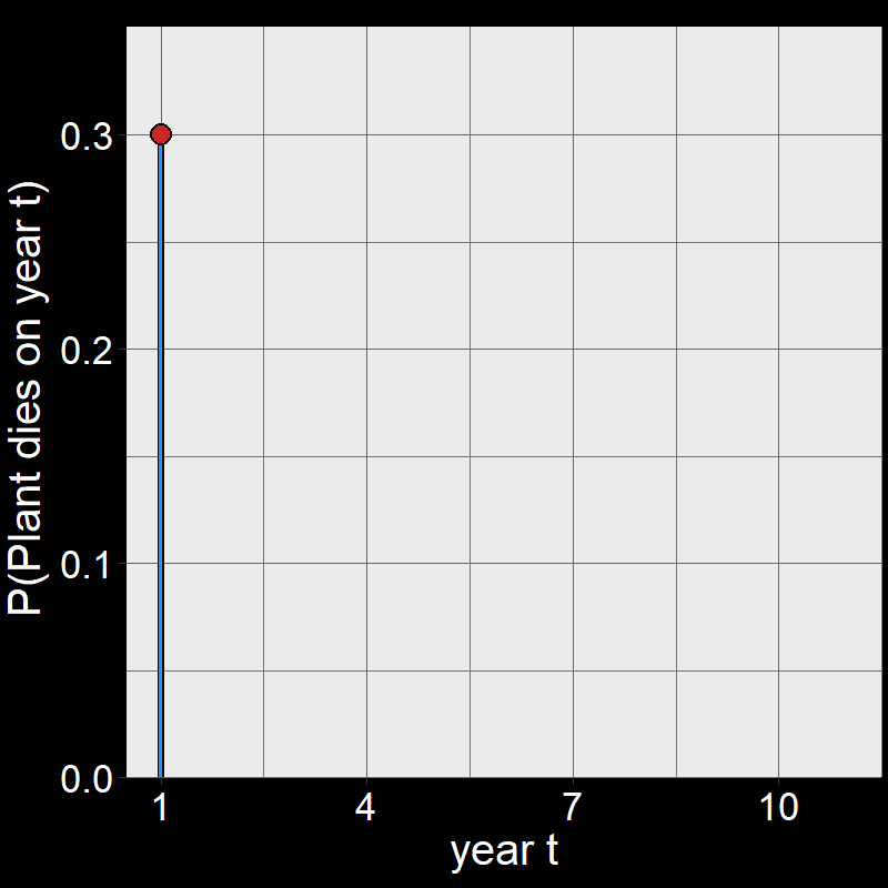
Perhaps surprisingly, plants are most likely to die on year \(t=1\).
Now, let’s see what we discussed above in action with the plant model and think about the average number of years plants live.
Let’s imagine a group of \(45\) plants, each of which die with probability \(\text{d}=0.3\) each year. If we let the dynamics of these plants unfold, it would look like this:

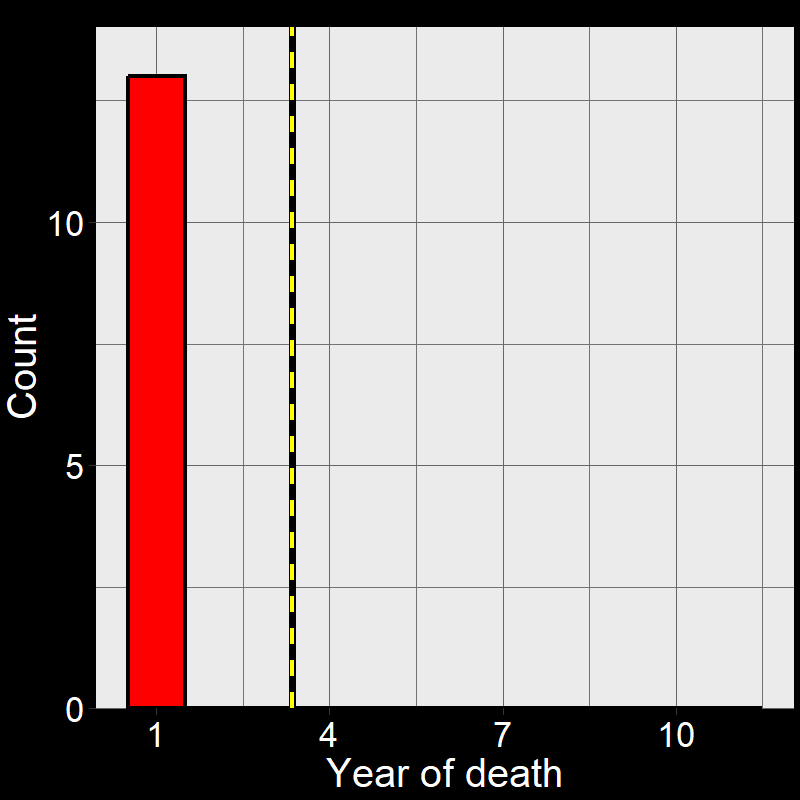
Figure 2.5A shows the life of each of the \(45\) plants (up until the time of death). Figure 2.5B shows a histogram of these time of death. Notice that the shape of the histogram notices the plot in Question 11D. The yellow and black line shows the average number of years plants live. As it so happens, the average year of death (i.e., average lifespan) of plant are: \(\overline{\text{lifespan}}= 3.35 \approx \frac{1}{0.3} = \frac{1}{\text{d}}\).
\(\qquad\) Using the geometric distribution, how does on show that \(\overline{\text{lifespan}}= \frac{1}{\text{d}}\). For those interested, see the derivation below. There are many way to solve it (and I may or may not have asked my favorite AI to help me write it…)
- What is a geometric distribution?: The geometric distribution models the number of “trials” needed to get the first “success”. Here, a “trial” is a year, where is a probability \(\text{d}\) of death;the “success” is a death event (although the term “success” seems a little questionable here). From before, we have:
\[ P(\text{death on year } t) = (1 - \text{d})^{t-1} \text{d} \]
- Expectation/average/mean of a geometric distribution: In our example, the average/mean of a geometric distribution (often called the “expectation”) is the average number of trials (years) needed to get the first success (plant death). Mathematically, the expectation \(E(Y)\) is:
\[\overline{\text{plant lifespan}} = E(\text{Years a plant lives}) = \sum_{t=1}^{\infty} t \cdot P(\text{death on year } t) \]
- Substitute P(eath on year t): Substitute the PMF into the expectation formula:
\[ E(\text{Years a plant lives}) = \sum_{t=1}^{\infty} t \cdot (1 - \text{d})^{t-1} \text{d} \]
- Factor out the probability of death: Factor out \(\text{d}\) from the summation:
\[ E(\text{Years a plant lives}) = \text{d} \sum_{t=1}^{\infty} t \cdot (1 - \text{d})^{t-1} \]
Simplify the summation: Recognize that the summation is a known series:
\[ \text{d} \sum_{t=1}^{\infty} t \cdot (1 - \text{d})^{t-1}\]
\(\qquad\) This series can be simplified using the formula for the sum of an infinite geometric series:
\[ \sum_{t=1}^{\infty} t \cdot r^{k-1} = \frac{1}{(1-r)^2} \]
\(\qquad\) where \(r = 1 - \text{d}\). Substituting \(r = 1 - \text{d}\) yields:
\[ \sum_{t=1}^{\infty} t \cdot (1 - \text{d})^{t-1} = \frac{1}{\text{d}^2} \]
- Combine the terms: Combine the results to get the expectation:
\[ E(\text{Years a plant lives}) = \text{d} \cdot \frac{1}{\text{d}^2} = \frac{1}{\text{d}} \]
\(\qquad\) This is one of many ways of showing the average plant lifetime is \(\frac{1}{\text{d}}\).
So! Those are the basics of geometric growth. This is not exhaustive, but it’s a start.
2.2.2 Exponential growth per se
The exponential growth model is essentially the continuous time version of geometric growth. By continuous time, I mean the model can deal with population changes from time \(t\) to \(t+\Delta t\), where \(\Delta t\) is any amount of time. This contrasts with the geometric growth model, which only deals in discrete pockets of time, \(t\) to \(t+1\).
\(\qquad\) Why might we want to think in terms of continuous time instead of discrete time? We’ll cover several reasons, but (as we will explore below) one issue is that discrete time can be a bit confusing in models. To exemplify this, let’s consider an alternative geometric growth model.
\(\qquad\) Consider the following model that is similar to the one we analyzed in the previous section. Each timestep of the model, three things happen (in this order):
- Reproductive adults produce seeds (as before)
- The seeds become reproductive adults
- A proportion of reproductive adult die
Here’s an animation of a timestep of the model:
Question 12: Explain the difference between this model and the geometric growth model we examined in the previous section. Consult the animations, if necessary.
Answer: Here, the order of events has changed.
Before, the reproductive adults died before the seeds became reproductive adults. Here, the seeds become reproductive adults before deaths, which means some of the new adults may die. This changes things a bit.
Question 13: For the model described in the above question, derive the equation for \(N(t+1) = ?\) and \(\lambda\). Is it the same or different from what we assumed above?
Answer:
Similar to before, we have \(\text{b} N(t)\) births. However, a proportion of \(\text{d}\) die each time-step. Thus, \[ \text{Increase} = \text{b} \times \big(1-\text{d}\big) \times N(t) \tag{2.9}\] Different from last time, only a fraction \(\big(1-\text{d}\big)\) will be counted for the adult stage. This is because deaths occur after the seeds become adults.
Identical to before we have \[ \text{Decrease} = \text{d} \times N(t) \tag{2.10}\] on the basis that a fraction \(\text{d}\) die. Putting these together, we get:
\[ N(t + 1)= N(t)\big(1 + \text{b} -\text{d} - \text{b}\text{d} \big) \tag{2.11}\]
which has this pesky additional \(\text{b}\text{d}\) term that represents the new individuals that die. Similarly, this means
\[ \lambda = 1 + \text{b} -\text{d} - \text{b}\text{d} \]
For a discrete-time model, the order of events each timestep changes the model a bit. This can be rather annoying, especially in more complex models.
\(\qquad\) Furthermore, populations typically don’t change in rigid, discrete blocks of time (although organisms such as annual plants do). Instead, births and deaths can generally at any time, occurring continuously through time; the idea that all individuals give birth and then some portion die (or vice versa) is questionable.
\(\qquad\) In contrast to discrete-time geometric growth, the (continuous-time) exponential growth model sidesteps this issue. How does exponential growth per se work, and how should you think about it? I will explain how I think about it, and (below) I’ll also provide what one typically is exposed to.
\(\qquad\) Let’s start with the assumption that individual plants have two things they do in life: give birth and die (they live wonderful lives). Specifically, individuals have a per capita birth death rate \(\text{b}\) (e.g., average births per unit time) and a per capita death rate \(\text{d}\) (deaths per unit time). If a plant gives birth, the seed it produces immediately turns into another reproductive adult plant. As time passes, individuals can spontaneously give birth or spontaneously die (imagine you’re waiting at a bus stop; you expect buses to come at a given rate based on their schedules, but some buses will randomly show up early or late). How long it takes until an event occurs (birth or death) and which one happens depends on the magnitudes of the rates \(\text{b}\) and \(\text{d}\).
Let’s see what this looks like:
In the figure above, the population generally increases over time. However, occasional decreases occur due to random death events.
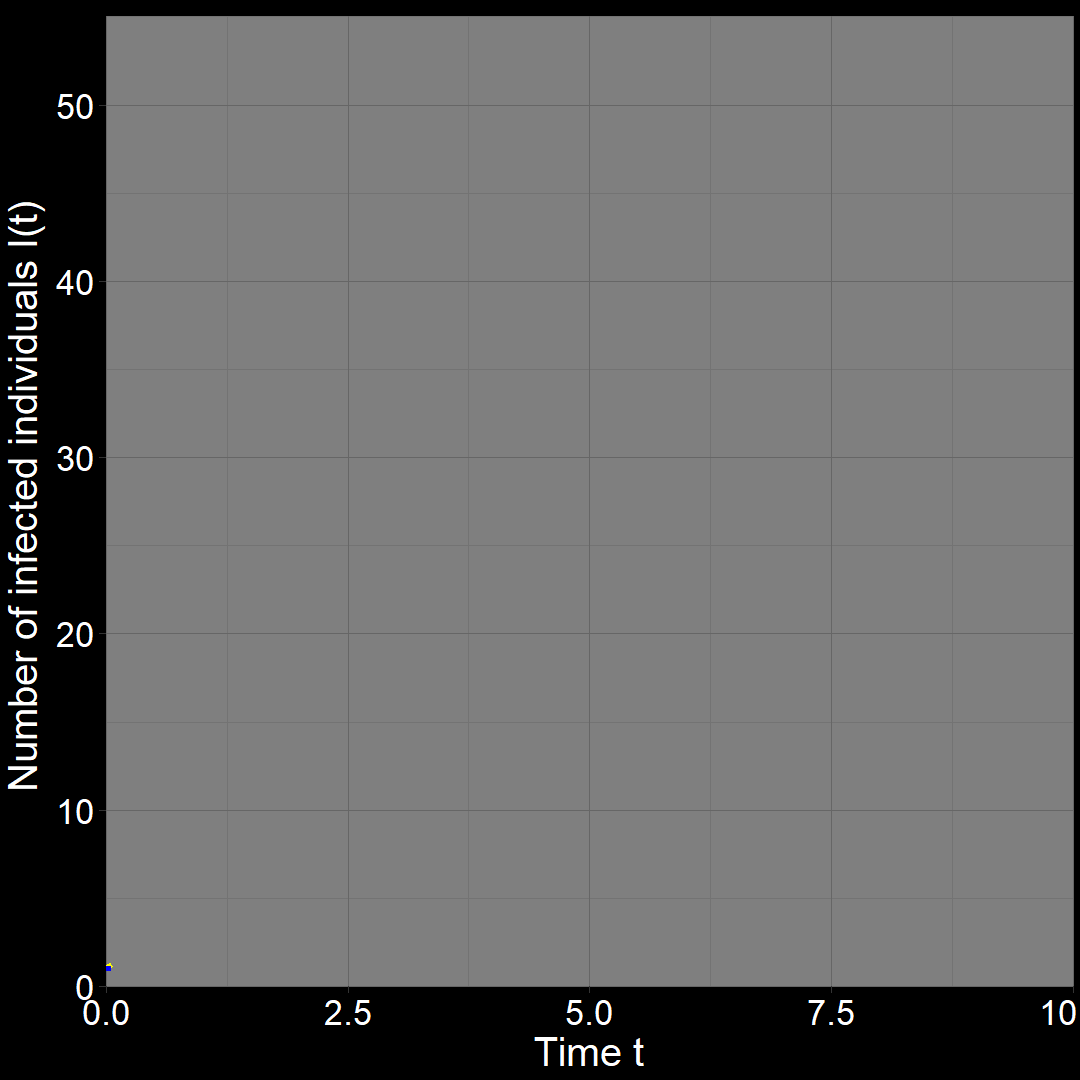
\(\qquad\) What do we expect to happen on average? The classic exponential growth model actually describes the average population trajectory predicted by the above model (if we were to run the model many times). Let’s visualize this:
\(\qquad\)The classic exponential model (blue) represents the average trajectory of the simulations (red). Each red squiggle depicts a different simulation of a population starting with \(10\) plants. While the squiggles generally follow the same direction, they vary due to random birth and death events. The blue curve, representing the classic exponential growth model, describes the average trajectory.
\(\qquad\) On average, individuals produce b offspring (seeds) per unit time and die at a rate of d per unit time. Thus, the total per capita rate of change is b - d. Consequently, the total change is \((\text{b} - \text{d})N(t)\). using this, the exponential growth model tells us the average rate at which the population changes at time \(t\). This is captured by the following equation:
\[ \underbrace{\frac{dN(t)}{dt}}_{\begin{array}{c}\text{The rate at which the} \\ \text{population is changing} \\ \text{at time } t\end{array}} = \underbrace{(\text{b} - \text{d})}_{\begin{array}{c}\text{per capita} \\ \text{growth}\end{array}} \times \underbrace{ N(t) }_{\text{abundance}} \tag{2.12}\]
This is the exponential growth model. Technically, it is an differential equation model.
Question 14A: What range of values can \(\text{b}\) take?
\[ 0 \leq \text{b} < \infty \]
\(\text{b}\) can take any non-negative value (on the basis that negative births aren’t possible).
Question 14B: What range of values can \(\text{d}\) take?
\[ 0 \leq \text{d} < \infty \]
Unlike the geometric growth model, \(\text{d}\) is no longer a proportion that dies within a give period of time; \(\text{d}\) is a rate per unit time. Therefore, \(\text{d}\) the rate can take any positive value (obviously, negative deaths don’t make sense unless resurrection is somehow involved).
\(\qquad\) As we will explore in a question below, if you know the death rate \(\text{d}\), you can calculate the proportion of the population that would die between time \(t\) and \(t + \tau\). The difference between the \(\text{d}\) in the exponential growth model and the \(\text{d}\) from the geometric growth model can be confusing (especially because they both use the same symbol \(\text{d}\).
Question 15: Explain the difference between exponential growth differential equation Equation 2.12 and the equation for geometric growth Equation 2.4. (Not formally, just the different information they provide).
Answer: The geometric growth equation describes the amount by which the population change in abundance over a fixed period of time (e.g. \(1\) year). Formally, this is called a difference equation AKA a recurrence relation.
In contrast, exponential growth, defined by a differential equation, describes how the rate at which the population changes at a given time.
For the exponential growth model, we often define
\[ r = \text{b}-\text{d} \]
where \(r\) is often called the “intrinsic rate of increase” or “intrinsic growth rate”. It is alternatively called the “Malthusian parameter of population growth”. This gives:
\[ \underbrace{\frac{dN(t)}{dt}}_{\begin{array}{c}\text{The rate at which the} \\ \text{population is changing} \\ \text{at time } t\end{array}} = \underbrace{\;r\;}_{\begin{array}{c}\text{intrinsic} \\ \text{growth rate}\end{array}} \times \underbrace{ N(t) }_{\text{abundance}} \tag{2.13}\]
Furthermore, we often represent Equation 2.13 as:
\[ \frac{1}{N(t)}\frac{dN(t)}{dt} = r \] We often then refer to the left hand side of the equation as the per capita growth rate of population \(N\). In the case of exponential growth, the per caipita growth rate is always equal to \(r\) – this will not be true in more complicated models.
\(\qquad\) From this equation, if we know \(r\) the population abundance at time \(t=0\) (\(N(0)\)), then we can calculate how much the population will change from time \(0\) to time \(t\). We get this by “solving” the differential equation, yielding:
\[ N(t) = N(0) e^{rt} \tag{2.14}\]
which is very similar to the our geometric growth model (see Equation 2.8). See “How to solve the differential equation” below.
Population increase and decrease for exponential growth
It is essential that you understand whether a population increases or decreases. This is simple, but fundamental:
Question 16A: Express the condition under which the population increases in terms of \(r\).
\(r >\)
Question 16B: Express the condition under which the population decreases in terms of \(r\).
\(r <\)
Question 16C: Express when the population will increase in terms of \(\text{b}\) and \(\text{d}\):
\(>\)
Question 16D: Rewrite the above in terms of b/d. That is, the population will increase when:
\(\frac{\text{b}}{\text{d}} >\)
Question 16E: What does \(\frac{\text{b}}{\text{d}}\) represent? (This question might sound familiar!)
\(\frac{\text{b}}{\text{d}}\) represents the average number of offspring (seeds) that an individual produces in their lifetime (i.e., the average number of births that occur per death in the population).
To see this consider the units of \(\text{d}\), which is \(\frac{\text{deaths}}{\text{unit time}}\). For simplicity, lets say \(\text{d}\) is in units \(\frac{\text{deaths}}{\text{year}}\). Then, \(\frac{1}{\text{d}}\) is in units \(\frac{\text{years}}{\text{death}}\) – in other words, \(\frac{1}{\text{d}}\) is the average amount of time (years) that individuals live.
Then, recalling \(\text{b}\) is in units \(\frac{\text{births}}{\text{unit time}}\) which, in this case, would be \(\frac{\text{births}}{\text{year}}\), we can see that
\[\begin{split} \frac{\text{b}}{\text{d}} & = \text{b} \times \frac{1}{\text{d}} \\ & = \bigg(\frac{\text{b births}}{\cancel{\text{year}}}\bigg) \times \bigg(\frac{1}{\text{d}} \frac{\cancel{\text{years}}}{\text{death}} \bigg) \\ & = \frac{\text{b}}{\text{d}} \frac{\text{births}}{\text{death}} \end{split}\]Hence, \(\frac{\text{b}}{\text{d}}\) is the average number of offspring (births) the average individual produces during their lifetime. Often, we represent
\[ R_0 = \frac{\text{b}}{\text{d}} \] where we call \(R_0\) (“arr-naught”) the “net reproduction rate”.
Question 17: John went and measured a population of trees that no longer reproduces (i.e., \(\text{b}=0\)). John found that by year \(t=3\) year (after three years), \(30\%\) of the trees had died. Assuming exponential decline, what is the annual death rate \(\text{d}\) (i.e., the \(\text{d}\) in Equation 2.12)?
We start with an initial number of \(N(0)\) trees. after \(3\) years, we have \(N(3) = 0.7 N(0)\) trees.
Then, use the fact that \(N(t) = N(0) e^{(\text{b}-\text{d})t}\) and our value of \(\text{b}=0\).
We have
\[ N(3) =0.7 N(0) \] Then, using \(N(t) = N(0) e^{rt}\) for \(t=3\) and plugging in \(N(3) =0.7 N(0)\), we get
\[ 0.7 N(0) = N(0) e^{(\text{b}-\text{d})3}\]
Recalling that \(\text{b}=0\) then gives us
\[0.7 N(0) = N(0) e^{-3 \, \text{d}}\]
Dividing each side by \(N(0)\) then gives us:
\[ 0.7 = e^{-3 \,\text{d}} \] which can be solved by taking the natural log of each side. Solving for \(\text{d}\) gives per capita death rate:
\[ \text{d} = \frac{-\log 0.7}{3} \approx 0.119 \; \; \text{deaths per year} \]
2.2.3 Questions on exponential and geometric growth
It is common practice to take the natural logarithm (\(\log\)) of population abundances for an exponentially growing population and fit a linear regression model of population growth through time:
![]()
In fact, geometric and exponential growth is always linear on the log scale. Let’s unpack that a bit.
Question 18A: In the above plots, what is the slope of the line? Express in terms of (1) r and (2) λ (copy and paste the λ symbol)
Try taking the \(\log\) of each side of the equation of Equation 2.14 and Equation 2.8, respectively.
Answer (1):
Answer (2):
Question 18B: With the above in mind, what is the relationship between r and λ?
\[ r = \log \lambda \]
Question 18C: Earlier, we derived the expression \[ N(t) = N(0) \lambda^t \] From this expression, write an expression for \(\lambda\).
First, divide each side by \(N(0)\): \[ \lambda^t = \frac{N(t)}{N(0)} \] and then thake the \(t_{\text{th}}\) root: \[ \lambda = \bigg(\frac{N(t)}{N(0)}\bigg)^{1/t} \]
Question 18D: Given the above two answers, imagine we again have \[ N(t) = N(0) \lambda^t \] From this expression, write the expression for \(r\).
First, divide each side by \(N(0)\): \[ \lambda^t = \frac{N(t)}{N(0)} \] and then thake the \(t_{\text{th}}\) root: \[ \lambda = \bigg(\frac{N(t)}{N(0)}\bigg)^{1/t} \] And, given that \(r = \lambda\), \[ r = \log\big(\lambda\big) = \log\bigg[\bigg(\frac{N(t)}{N(0)}\bigg)^{1/t}\bigg] = \frac{1}{t}\log\bigg[\frac{N(t)}{N(0)}\bigg] \]
Question 19: With answers of the above question in mind, imagine you know the abundance of a population at two times, \(t\) and \(t + 1\). Thus, you have \(N(t)\) and \(N(t + 1)\). You know the population growing geometrically/exponentially. How would you calculate \(r\) from these two values?
Think of calculating slope as you would calculate from \(y = mx + b\) from two points.
\[ r = \frac{\ln \big[ N(t + 1)\big] - \ln \big[N(t)\big]}{(t + 1) - 1} = \ln \bigg[\frac{N(t + 1 )}{N(t)}\bigg] \]
This an important result; numerous empirical studies (especially those study the growth of bacteria) use this formula to calculate \(r\).
Above, the models has been rather abstract. Below, we will explore exponential growth applied to the spread of an infectious disease.
Exponential growth during the initial spread of an infectious disease
As we discussed above, the initial spread of a pandemic is often exponential (e.g., COVID-19). Where does this exponential growth come from?
\(\qquad\) Interestingly, the simplest epidemiological models in ecology approach diseases indirectly – we don’t model the disease itself but rather the number of individuals infected by it. Thus, our “disease” population is represented by the density (or abundance) of \(I\)nfected individuals at time \(t\), denoted as \(I(t)\).
\(\qquad\) Let’s assume we’re in the beginning of a pandemic, so we have an initial population of \(N\) individuals that are susceptible to the disease. For simplicity, let’s assume \(N\) is constant, meaning the “susceptible pool” never decreases. This is a reasonable assumption for the initial stages of an epidemic. With these assumption, we can describe the following model:
\[ \frac{dI(t)}{dt} = \underbrace{\beta N I(t)}_{\substack{\text{total} \\ \text{infection}\\ \text{rate} } } - \underbrace{\gamma I(t)}_{\substack{\text{total} \\ \text{recovery}\\ \text{rate} } } \tag{2.15}\]
where
- \(\beta\) is the per capita rate of infection (how quickly infected individuals infect healthy individuals)
- \(N\) is the number of individuals susceptible to infection (that we, for simplicity, assume is constant)
- \(I(t)\) is the number of infected individuals at time \(t\)
- \(\gamma\) is the recovery rate (how quickly infected individuals get better)
What is this model saying? We’ll explore the mechanics of this and similar models more deeply later. The idea is that infected individuals \(I(t)\) “bump into” the \(N\) susceptible individuals at a rate \(\beta\), infecting them. Meanwhile, individuals recover from sickness at a rate \(\gamma\). Roughly, the model approximates what is shown in the figures below:
With this in mind, let’s examine the initial exponential growth of an epidemic.
What are equivalent to per capita birth rate \(\text{b}\), death rate \(\text{d}\), and the intrinsic rate of increase \(r\) for Infected individuals in Equation 2.15?
Question 20A: fill in the blank. \(\text{b}= \_\_\_\_\_\_\)
\[ \text{b} = \beta N \]
Question 20B: fill in the blank. \(\text{d} = \_\_\_\_\_\_\)
\[ \text{d} = \gamma \]
Question 20C: fill in the blank. \(r = \_\_\_\_\_\_\)
\[ \text{intrinsic rate of increase: }\;\; r = \beta N - \gamma \]
These quantities are the key understanding if/when a disease spreads through a population.
Let us again assume that the disease is very rare in the population. Under what circumstance would it increase when rare? Express this in two ways:
Question 21A: fill in the blank. The disease increases when rare when ______ \(> 0\)
\[ \beta N - \gamma >0 \]
Identical to classic exponential growth model, the population grows if \(b-d>0\).
Question 21B: fill in the blank. The disease increases when rare when ______ \(> 1\)
See question 16D
\[ \frac{\beta N}{\gamma } >1 \]
This is easily rearranged from \(\beta N - \gamma >0\).
In epidemiology, \(\frac{\beta N}{\gamma}\) (and other similar quantities) is known as \(R_0\) (pronounced “arr-naught”). This \(R_0\) is conceptually and mathematically identical to the \(R_0\) we discussed in question 16E. \(R_0\) is often referred to as the “basic reproduction number” in epidemiology (in contrast to “net reproduction rate” in population biology/ecology).
\(\qquad\) Conceptually, \(R_0\) represents the number of susceptible individuals that one infected individual is expected to infect over the course of their illness. This makes sense when you break down each term: \(\beta N\) is the rate of infection, and \(1/\gamma\) is the average duration of infection (essentially, “one divided by the rate at which infections end”). Therefore, \(R_0 = \frac{\beta N}{\gamma}\) is the infection rate multiplied by the length of time that infection can occur, giving the total number of infections.
\(\qquad\) Please play around with this Shiny interactive web app, Module 2.3. In this module, you can explore the trajectory of the number of infected individuals \(I(t)\) for different values of \(\beta N\) and \(\gamma\). Notice what happens when e.g. \(R_0 = \beta N/\gamma<1\).
\(R_0\) is a very famous quantity – it even made an appearance in Hollywood! The concept was explained by Kate Winslet in Steven Soderbergh’s 2011 feature film Contagion:
Of course, we’re in a post-COVID world, so perhaps you already knew about \(R_0\).
Notably, Kate mentions a few things that we didn’t include in our model (e.g. the incubation period). There are a very large number of models that calculate \(R_0\) in different ways – each of these models adds different biological details.
2.3 \(R_0\) vs \(\lambda\) and \(r\)
In the previous sections, we discussed \(\lambda\) and \(r\) (the finite rate of increase and the intrinsic growth rate, respectively). We also explored another common measure of population growth, the net reproductive rate \(R_0\) (see Question 16E), which is referred to as the basic reproduction number in epidemiology.
\(\qquad\) As mentioned earlier, the net reproductive rate is typically defined as the average number of offspring an individual produces during its lifetime (note: many definitions specify \(R_0\) as the number of daughters a female produces, but we’ll ignore this distinction for now).
\(\qquad\) We previously noted the similarities between \(\lambda\) and \(r\). So, how does \(R_0\) differ from \(\lambda\) and \(r\)?
2.3.1 \(r\) vs. \(R_0\)
Let’s start with a question. Recall the disease model from Equation 2.15 (if you haven’t done the questions associated with that section, please do them before moving forward).
You are part of disease control group, analyzing the danger of two diseases, disease \(A\) and disease \(B\). You are concerned about how quickly each disease initially spreads. For disease \(A\), you have measured \(R_0 = \beta N/ \gamma= 5\) (see Question 21B). That is all you know about disease \(A\). For disease \(B\), you know \(r=0.4\) (i.e., \(r_B =\beta N - \gamma = 0.4\); see Question 21A). That is all you know about disease \(B\).
Question 22A: Which quantity do you need to compare between the diseases to see which disease initially spreads more rapidly?
The rate at which a population increases is given by the intrinsic rate of increase \(r = \beta N - \gamma\). Thus, we need to compare the intrinsic rate of increase of disease \(A\), \(r_A\), with that of disease \(B\), \(r_B\).
Question 22B: Which disease do you expect to spread more rapidly? Justify your answer.
Play around with this interactive Shiny app, Module 2.3.
Try picking different values of \(\beta N\) and \(\gamma\) that satisfy \(R_0 = 5\). What values of \(r_A = \beta N - \gamma\) does it yield? How do these values compare to \(r_B = 0.4\)?
There is not enough information provided to answer if disease \(A\) or \(B\) will spread faster. This is because the net reproductive rate / basic reproduction number \(R_0\) and intrinsic growth rate \(r\) contain different information.
Here is an in-depth explanation.
Since we’re worried about how quickly the disease spreads, the quantity of interest is \(r = \beta N - \gamma\). For disease \(B\), we know \(r_B = 0.4\). But what is \(r_A\) for disease \(A\)? As it turns out, we can’t say. Let’s go through some examples by considering the \(R_0\) for disease \(A\), for which \(R_0 = \frac{\beta N}{\gamma} =5\). What can we say about \(r_A = \beta N - \gamma\)?
Assuming \(R_0 = 5\), it could be that \(\beta N =5\) and \(\gamma=1\). This gives \(r_A = \beta N - \gamma = 5-1=4\). In this case, disease \(A\) would spread \(10\) times faster than disease \(B\).
Alternatively, let \(\beta N =0.5\) and \(\gamma=0.1\). Once again, \(R_0 = 5\), but now \(r_A = \beta N - \gamma = 0.5-0.1=0.4\). In this scenario, diseases \(A\) and \(B\) spread at the same rate.
It’s just as possible that \(R_0 = 5\) because \(\beta N =0.05\) and \(\gamma=0.01\). Now, \(r_A = \beta N - \gamma = 0.05-0.01=0.04.\) In this scenario, diseases \(A\) spreads \(10\) times slower than disease \(B\).
In fact, there are an infinite number of values that work. Let \(\beta N =0.65\) and \(\gamma=0.13\). Once again, \(R_0 = \frac{0.65}{0.13}= 5\) while \(r_A = \beta N - \gamma = 0.5-0.1=0.52\). Here, \(A\) spreads slightly faster than \(B\).
Below, these cases are depicted:
Try it yourself!
You can also check these values yourself using this interactive Shiny app, Module 2.3.
\(\qquad\) In other words, disease \(A\) (with its \(R_0 = 5\)) could grow \(10\) times faster than disease \(B\), the same rate as disease \(B\), \(10\) times slower than disease \(B\) or at literally at any positive rate. We cannot determine anything about how quickly disease \(A\) spreads just from the \(R_0\).
\(\qquad\) This is not merely a mathematical result. For example, let’s consider two diseases: (1) season flu and (2) HIV. Seasonal flu has an estimated \(R_0\) between \(1-2\) (Biggerstaff et al. 2014) while historical estimates of \(R_0\) for HIV have been between 2-5 or even higher in sub-Saharan Africa (Williams and Gouws, 2014), although estimates obviously depend on the context. Despite a larger \(R_0\), we all intuitively know that HIV spreads much less rapidly than flu. This is because people who are infected with HIV (at least, at the time of writing this) typically remain infected their entire lives, in which case, an individual infected with HIV may infect several people over several decades. In contrast, people spread flu fairly rapidly, but can only infect others for a week or two. Thus, we cannot rely on measurements of \(R_0\) to say how quickly a disease spreads.
\(\qquad\) Confusion between \(R_0\) and \(r\) (or \(\lambda\)) is common, even in the media. For example, let’s pick on NPR:
Question 23: Consider this quote from an NPR article about an Ebola outbreak back in 2014::
…Take, for example, measles. The virus is one of the most contagious diseases known to man. \(R_0\) sits around \(18\). That means each person with the measles spreads it to \(18\) people, on average, when nobody is vaccinated… At the other end of the spectrum are viruses like HIV and hepatitis C. Their \(R_0\)s tend to fall somewhere between 2 and 4. They’re still big problems, but they spread much more slowly than the measles.
Did NPR use \(R_0\) appropriately in the above quote? Explain.
NPR is not wrong that measles spreads more rapidly than HIV and hepatitis C. However, one cannot use \(R_0\) to determine the rate at which a disease spreads. Therefore, the quote is potentially misleading because \(R_0\) does not give information about the rate of growth – \(r\) does.
\(\qquad\) To be fair to NPR, however, they were apparently informed of this issue – they added this in a footnote:
The \(R_0\) is integrated over the time that a person is infectious to others. For HIV, this could be years. But for Ebola, that time is only about a week. So even though they have similar \(R_0\)s, Ebola’s infections per unit of time is much higher than HIV’s.
However, unless one actually reads the footnote, one would walk away with the mistaken impression that a disease with a larger \(R_0\) will spread faster. Am I being persnickety? You bet.
It is therefore important to keep in mind that \(R_0\) and \(\lambda\) / \(r\) provide different information.
Question 24: For discrete-time growth, Equation 2.6 and Equation 2.8, there is a special situation in which \(R_0 = \lambda\) and, therefore, \(\lambda\) and \(R_0\) provide the same information. What is this situation?
Think about \(\lambda\) in terms of \(\text{b}\) and \(\text{d}\), and pick a value of \(\text{d}\) gives you the desired result.
This occurs for “non-overlapping generations” (i.e, when \(\text{d}=1\) for the geometric growth model such that all members of the population die each time step after reproducing). An example would be an annual plant.
If an individual always dies after reproducing, then its reproductive output is \(\lambda = b\) per lifetime. Thus, if we know \(\lambda\), we know \(R_0\) and vice versa. Identically, we also know that \(r = \log \lambda = \log R_0\).
This is the only situation in which this occurs. Otherwise, \(r\) / \(\lambda\) and \(R_0\) provide different information.
2.4 Stage structure
One thing that might concern you about our geometric/exponential growth plant models is that we only track “adults.” In our plant model, we assumed all seeds turn into reproductive adults at the end of each time step (see video 1). In our continuous time (exponential growth) model, seeds effectively become adults immediately. But what happens if it takes time for a seed to grow into an adult? Let’s explore this with a new model.
2.4.1 Building the stage structured model
In our new model, only a proportion of seeds \(\text{g}\) mature each timestep. Previously, we managed by tracking only the number of reproductive adults (\(N(t)\)). However, this approach won’t suffice for our new model. We now need to keep track of both reproductive adults \(A(t)\) and seeds, which we’ll refer to as juveniles \(J(t)\). In equation form, this looks like:
\[\begin{split} & J(t+1) \: = J(t)\; + \text{ increase}_{J(t)}\; - \text{ decrease}_{J(t)} \\ & A(t+1) = A(t) \;+ \text{ increase}_{A(t)} \; - \text{ decrease}_{A(t)} \end{split}\]where \(\text{increase}_{A(t)}\) and \(\text{decrease}_{A(t)}\) represents the increase/decrease in the number of adults each timestep, and \(\text{increase}_{J(t)}\) and \(\text{decrease}_{J(t)}\) represents the increase/decrease in the number of juveniles (seeds) each timestep.
\(\qquad\) We refer to a model with multiple life history stages (e.g., juveniles and adults) as a “stage-structured” model.
\(\qquad\) Now, like any good modeler, we need to make some assumptions. Will these assumptions be bulletproof? No, of course not. But that’s how it goes – we dream up models and then we critique their assumptions.
Here are the assumptions of our new model:
- Each adult produces \(\text{b}\) juveniles (seeds) per timestep.
- A proportion \(\text{d}\) of adults die each timestep.
- Adults can reproduce; juveniles cannot.
- Each timestep, a proportion of seeds \(\text{g}\) grow/mature into reproductive adults.
- Seeds do not die (not super realistic, of course, but we’re trying to add one thing at a time).
- Each timestep, the order of events is as follows: (1) adult reproduction, (2) adult death, (3) juveniles (seeds) grow into reproductive adults.
Try to picture or draw how the model works. I think it’s helpful to see the model in action.
Using this, let’s fill in expressions of the model.
For the following questions, fill in the blanks. Keep in mind the order of events.
Question 25A: \(\text{ increase}_{J(t)}=\) ______ ?
\[ \text{ increase}_{J(t)} = \text{b}A(t) \tag{2.16}\]
This one is relatively straightforward; we have births into the juvenile class.
Note: you could also have written
\[ \text{ increase}_{J(t)} = (1-\text{g})\text{b}A(t) \] which would take into account the fact that a proportion of the needs seeds \(\text{g}\) germinate each timestep.
Question 25B: \(\text{ decrease}_{J(t)}=\) ______ ?
\[ \text{ decrease}_{J(t)}= \text{g} J(t) + \text{g} \text{b} A(t) \tag{2.17}\]
A proportion $ J(t)$ of the already-present juveniles grow into reproductive adults ; a proportion \(\text{g} \text{b} A(t)\) of the newly-born juveniles also grow into reproductive adults.
Alternatively, you could have written \(\text{g} J(t)\)
\[ \text{ decrease}_{J(t)}= \text{g} J(t) \tag{2.18}\]
if you wrote \(\text{ increase}_{J(t)} = (1-\text{g})\text{b}A(t)\) above.
Question 25C: \(\text{ increase}_{A(t)}=\) ______ ?
\[ \text{ increase}_{A(t)}= \text{g} J(t) + \text{g} \text{b} A(t) \]
This accounts for all the juvenile seeds (both old and newly born) that grow into reproductive adults.
Question 25D: \(\text{ decrease}_{A(t)}=\) ______ ?
\[ \text{ decrease}_{A(t)} = \text{d} A(t) \]
Adults die; pretty straightforward.
Using the answers to the above questions, we have all the terms of our model.
Question 26: Using the answers from Question 25, substitute all “increase” and “decrease” values into
\[\begin{split} & J(t+1) \: = J(t)\; + \text{ increase}_{J(t)}\; - \text{ decrease}_{J(t)} \\ & A(t+1) = A(t) \;+ \text{ increase}_{A(t)} \; - \text{ decrease}_{A(t)} \end{split}\]so what we get our new model.
There are several ways to combine the terms. Here is what I did:
\[ \underbrace{J(t + 1)}_{\begin{array}{c}\text{Juveniles (seeds)} \\ \text{at year }t+1\end{array}} = \underbrace{\;\; (1-\text{g}) J(t) \; \;}_{\begin{array}{c}\text{seeds already present } \\ \text{ that don't mature}\end{array}} + \underbrace{\;\; (1-\text{g}) \text{b} A(t) \; \;}_{\begin{array}{c}\text{seeds born this timestep} \\ \text{that don't mature}\end{array}} \tag{2.19}\]
\[ \underbrace{A(t + 1)}_{\begin{array}{c}\text{Adults at} \\ \text{year }t+1\end{array}} = \underbrace{\;\; \text{g} J(t) \; \;}_{\begin{array}{c}\text{seeds already present} \\ \text{that mature}\end{array}} + \underbrace{\text{g} \text{b} A(t) \; \;}_{\begin{array}{c}\text{seeds born this} \\ \text{timestep that mature}\end{array}} - \underbrace{\big(1-\text{d}\big)A(t)}_{\begin{array}{c}\text{proportion of} \\ \text{Adults that die}\end{array}} \tag{2.20}\]
Make sure your answers are the same as Equation 2.19 and Equation 2.20, even if you didn’t write the equations in exactly the same way. If you made an mistake with the algebra, that’s okay! The key is to make sure that you understand why each term goes where.
Now that we have our model, it makes sense to follow the same approach we used for geometric growth. In our discrete-time geometric growth model, we derived:
\[ \frac{N(t+1)}{N(t)} = \lambda = 1+b-d \] where \(\lambda\) is our finite rate of increase. It seems like there should be some kind of equivalent expression for the stage-structured model described by Equation 2.19 and Equation 2.20. That is, we want:
\[ \frac{A(t+1) + J(t+1)}{A(t) + J(t)} \stackrel{?}{=} \lambda = \; ? \tag{2.21}\]
Wouldn’t it be nice to have a value analogous to \(\lambda\)? Surely, we should be able to find a way to measure the total growth of juveniles and adults. But how?
Question 27: How do you expect the finite rate of increase (\(\lambda\)) for our stage-structured model to differ in magnitude from the scenario of geometric growth where there was no juvenile stage, assuming all other factors remain equal?
\(\lambda\) should be…
If a seed does not become a reproductive adult in the same timestep it is produced, it has to “wait” before it can reproduce itself. This delay slows down the rate at which new individuals are added to the population, thereby decreasing \(\lambda\) compared to a scenario where all seeds immediately become reproductive adults.
In addition to \(\lambda\), we might be interested in knowing “how many juveniles (seeds) are there relative to reproductive adults?” Why might this be important? Let’s imagine we want to determine the number of seeds in the population. Counting seeds can be challenging, but counting adults is relatively easy. However, maybe we can calculate the number of seeds if we know the number of adults. How might we approach this?
2.4.2 Breaking the eigen-barrior: analyzing the model
To explore these concepts (\(\lambda\) and the ratio of juveniles to adults), we need to rewrite our model slightly differently (though entirely equivalently) using matrix notation:
\[ \begin{bmatrix} J(t + 1) \\ A(t + 1) \end{bmatrix}= \begin{bmatrix} (1-\text{g}) & (1-\text{g}) \text{b} \\ \text{g} & (1 + \text{g}\text{b} -\text{d}) \end{bmatrix} \begin{bmatrix} J(t) \\ A(t) \end{bmatrix} \tag{2.22}\]
where the “matrix” is:
\[ \begin{bmatrix} (1-\text{g}) & (1-\text{g}) \text{b} \\ \text{g} & (1 + \text{g}\text{b} -\text{d}) \end{bmatrix} \] This is called a \(2 \times 2\) matrix (it has two rows and two columns). In population biology, we refer to this as the “transition matrix” because it describes the transition between life stages (juvenile and adult stages). Take a moment to compare the terms in the above matrix with all the right-hand-side terms in Equation 2.19 and Equation 2.20 – they contain the same information.
Similarly,
\[ \begin{bmatrix} J(t) \\ A(t) \end{bmatrix} \] This is called a vector of length two. It is a convenient way to keep track of the abundances of juveniles \(J(t)\) and adults \(A(t)\).
Equation 2.22 is exactly the same as Equation 2.19 and Equation 2.20 (taken together). This animation should help clarify how to read the model in matrix form and convince you that they are indeed the same.
where the arrows imply multiplication. As can see, Equation 2.22 contains the same information as Equation 2.19 and Equation 2.20.
\(\qquad\) Why bother putting things in matrix form? While some people might find it neater, the real reason is that matrices have all sorts of useful mathematical properties we can take advantage of.
\(\qquad\) Enter a couple of intimidating words: eigenvalues and eigenvectors. Eigenvalues and eigenvectors are fundamental properties of “square” matrices (like the matrix above, which has 2 columns and 2 rows; matrices with the same number of columns and rows are called square). By “fundamental property” I mean something a little bit like how the roots and vertex of a quadratic are fundamental properties of a quadratic equation.
\(\qquad\) Our transition matrix describes how births, deaths, and seed growth/maturation affect adult and juvenile population changes. As it turns out, the eigenvalues and eigenvectors reveal how our adult and juvenile population abundances change.
\(\qquad\) Eigenvalues and eigenvectors can be confusing to learn about without a background in linear algebra. My teaching approach is as follows: instead of just “telling” you what eigenvalues and eigenvectors represent in our model, let’s see if we can visualize them. I will not delve into the mathematical details; see Otto and Day (2011), Primer 2 for an excellent and approachable reference.
2.4.3 Analysis when g = 1
Let’s start with something more basic. Let’s review the previous question:
Question 28: What happens to our stage-structured model \(\text{g}=1\)? (i.e., \(\text{g}=1\) is a special case of the model; what is that special case?)
When \(\text{g}=1\), the model with juveniles becomes identical to the geometric growth model lacking stage structure.
This is because, when \(\text{g}=1\), all juveniles always immediately become adults. Therefore (at least, after the first timestep) there will never by any juveniles to keep track of.
With the above in mind, let’s visualize our model with \(\text{b}=0.1\), \(\text{d}=0.05\), and \(\text{g}=1.0\). Perhaps eigenvectors and eigenvalues will reveal themselves in the process.
\(\qquad\) Consider the plots below. They show the outcomes of different simulations of the model, each starting with a different number of adults and juveniles. We are tracking the trajectory of the abundance of each.
\(\qquad\) First, let’s plot the population abundances for the adults and juveniles:
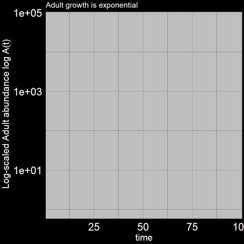
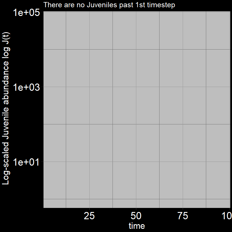
Because \(\text{g}=1\), all the juveniles always disappear after the first timestep; the adults grow exponentially (note the log-scaled y-axis).
Next, let’s consider the “direction” of population growth in terms of adults vs. juveniles over time. One effective way to visualize this is by plotting adults \(A(t)\) on the x-axis and juveniles \(J(t)\) on the y-axis:
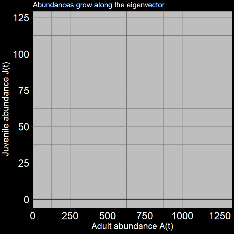
After the initial timestep (in which all juveniles become adults), we only move horizontally (in the direction of the adults). Again, this is because juveniles always transition into adults (\(\text{g}=1\)). Seems pretty simple, right? However, the black line in the plot (along which the arrows move) represents the eigenvector. (Technically, it is one of two eigenvectors – this eigenvector is associated with something called the “dominant eigenvalue” – don’t worry about that for now.)
\(\qquad\) The key point is that the population grows in the horizontal “adult direction.” Mathematically, we could describe this with:
\[ \text{eigenvector} = \mathbf{\nu} = \begin{bmatrix} 0 \\ 1 \end{bmatrix} \] where the “\(1\)” is in the adult \(A(t)\) direction and the “\(0\)” is in the juvenile (seed) \(J(t)\) direction. In short, the eigenvector tells us the direction the system moves (adult vs. juvenile directions) in the long run. Here, we only move in the adult direction. Things will get more interesting when \(\text{g}<1\).
\(\qquad\) Third, we might ask, “What proportion of the population are adults vs. juveniles?” This would be expressed as \(\frac{A(t)}{A(t) + J(t)}\).
Question 29: In light of the previous plot, what proportion of adults \(\frac{A(t)}{A(t) + J(t)}\) do you expect the system to reach?
Answer:
The below plot shows the ratio of adults to juveniles \(\frac{A(t)}{A(t) + J(t)}\) as time unfolds:
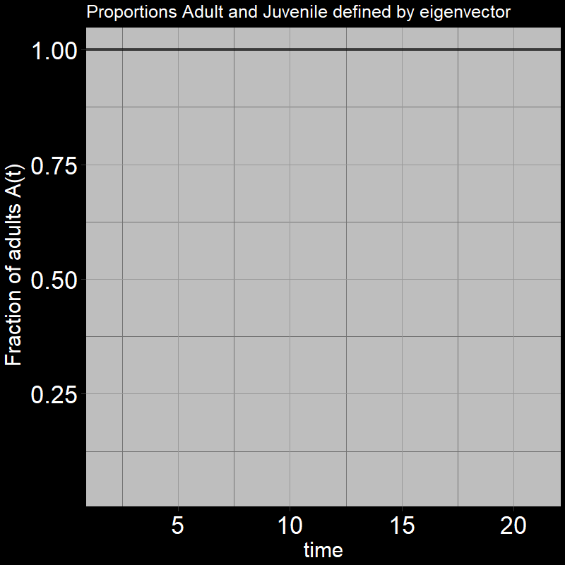
Indeed, the ratio quickly converges to \(\frac{A(t)}{A(t) + J(t)}=1\)
\(\qquad\) Fourth, we ask “how quickly does the population grow?”. The below plot depicts \(\frac{A(t+1) + J(t+1)}{A(t) + J(t)}\) each timestep of the model:
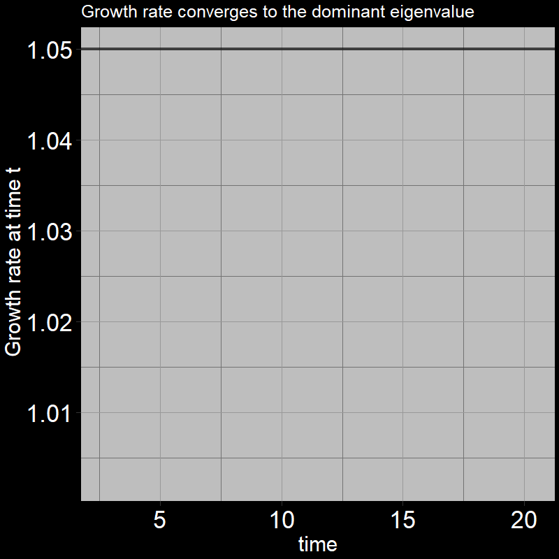
The black line shows the eigenvalue. (Technically, it is the “dominant” eigenvalue, the largest eigenvalue associated with the matrix; there are multiple eigenvalues / more to learn about… don’t worry about it for now!) .
\(\qquad\) After the first timestep, \(\frac{A(t+1) + J(t+1)}{A(t) + J(t)}\) converges to the dominant eigenvalue, which is equation to exactly \(1.05\).
Question 30: For our case of \(\text{g}=1\), what do you expect \(\lambda\) to be? I’m looking for analytical expression (not \(1.05\), given above)
Don’t try calculating things out / doing much math; think about how \(\text{g}=1\) affects the system. Think about \(\text{b}\) and \(\text{d}\).
\(\lambda\) will be the same as the original geometric growth model:
\[ \lambda = 1 + b -d \]
Recall \(\text{b}=.1\) and \(\text{d=.05}\). Thus, the dominant eigenvalue is \(\lambda = 1 + \text{b} - \text{d} = 1 + 0.1 - 0.05 = 1.05\). Hence, the eigenvalue tells “how quickly” things are growing.
2.4.4 Analysis when g < 1
We will perform the same analyses as above, but this time with \(\text{b}=0.1\), \(\text{d}=0.05\), and \(\text{g}=0.25\).
First, let’s consider the population growth of adults and juveniles. Because \(\text{g}<1\), some juveniles will indeed be present:
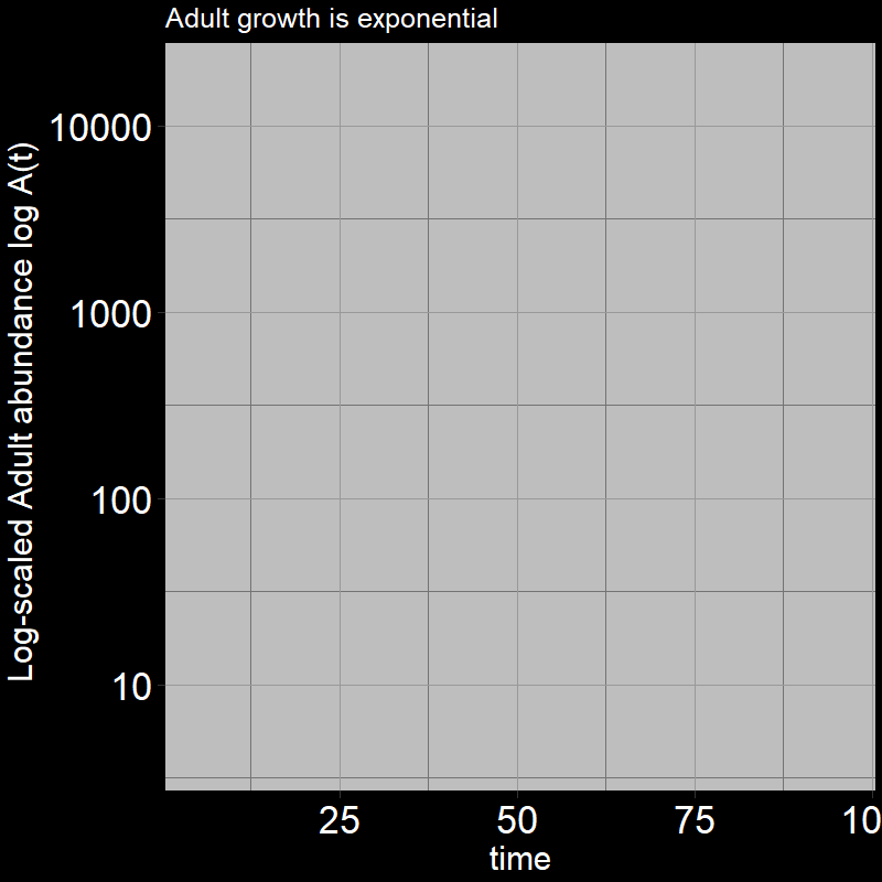
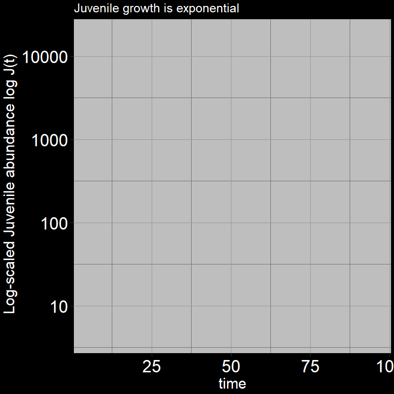
Both \(A(t)\) and \(J(t)\) have non-zero abundances, growing exponentially.
Second, let’s again consider the “direction” of population growth in terms of adults vs. juveniles over time. We visualize this is by plotting adults \(A(t)\) on the x-axis and juveniles \(J(t)\) on the y-axis:
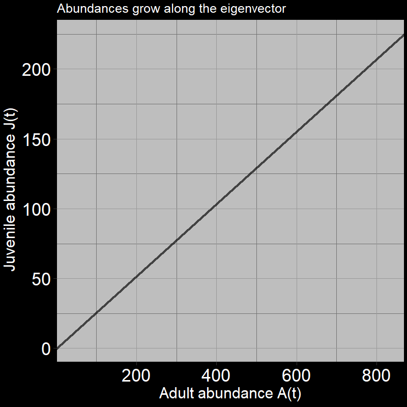
The system grows in a characteristic direction defined by the black line. The black line is, in fact, the eigenvector, where:
\[ \text{eigenvector} = \mathbf{\nu} = \begin{bmatrix} .25 \\ .97 \end{bmatrix} \]
In addition, for simplicity, we will associate each with a direction:
\[ \mathbf{\nu}[J] = .25 \; \; \text{ and } \; \; \mathbf{\nu}[A] = .97 \]
where \(A\) and \(J\) index the direction associated with the juvenile and adult directions, respectively.
Question 31A: Conceptually, what does the slope of the black line represent? Answer in terms of juveniles and adults.
As you should know by now, the black line is the eigenvector.
The slope of the black line represents the increase in adult abundance relative to juvenile abundance, as time passes.
Question 31B What is the slope of the black line (numerically)? Round to three digits (e.g. x.yz)
Answer:
We must simply calculate how much the adult increases relative to how much the juvenile increases. This is given by
\[\frac{\mathbf{\nu}[A]}{\mathbf{\nu}[J]} = \frac{.97}{.25} \approx 3.88\]
I personally think of the eigenvector in this context as the “path of least resistance defined by the transition matrix.” The transition matrix indicates the direction in which the relative magnitudes of births, adult deaths, and seed growth/maturation push the trajectory of juvenile and adult population abundance growth.
Try it yourself!
Examine the effect of modifying \(\text{g}\) on the eigenvector using this interactive Shiny app, Module 2.4.
Next, we again ask, “What proportion of the population are adults vs. juveniles?” This can be expressed as \(\frac{A(t)}{A(t) + J(t)}\).
As before, it converges to a particular value:
Question 32: What proportion of adults \(\frac{A(t)}{A(t) + J(t)}\) do you expect the system to reach in the long-term (as \(t\) gets large)? Round to three digits (e.g. 0.abc).
Answer:
Recall that the eigenvector indicates the relative growth of adults vs. juveniles. How might this affect the number of adults you would find relative to juveniles?
In the long-term (as \(t\) gets sufficiently large):
\[\frac{A(t)}{A(t) + J(t)} \rightarrow \frac{\mathbf{\nu}[A]}{\mathbf{\nu}[A]+\mathbf{\nu}[J]} = \frac{.97}{.97+.25} \approx 0.795\] As time passes, the population distributes itself among the different stages (juvenile and adult in your model) in proportions given by the components of the eigenvector corresponding to the dominant eigenvalue.
Fourth, and finally, let’s consider the overall growth of the system. Both the adult and the juvenile increase in abundance – but what is the overall amount of increase?
All trajectories converge to the same growth per timestep. The plot shows \(\frac{A(t+1) + J(t+1)}{A(t) + J(t)}\) on the y-axis:
In summary, in the long run, the population increases by a fixed proportion each timestep. For the simple (adult-only) geometric growth model, this proportion is \(\lambda=1+\text{b} -\text{d}\). The analogous quantity in our stage-structured model is the dominant eigenvalue of the transition matrix.
If you’re curious, this is what the dominant eigenvalue looks like:
\[ \lambda = \frac{1}{2} \left(2 + \text{b} \text{g}-\text{d}-\text{g} + \sqrt{(-\text{b} \text{g}+\text{d}+\text{g}-2)^2-4 (\text{d} \text{g}-\text{d}-\text{g}+1)}\right) \] noting we usually usually uses a \(\lambda\) to represent eigenvalues. Not so pretty, right? Bonus points if you can show that \(\lambda = 1+\text{b} -\text{d}\) when you take the limit of \(\text{g} \rightarrow 1\).
2.4.5 Continuous Time Stage-Structured Model
The continuous time stage-structured model, in matrix form, is quite elegant:
\[ \begin{bmatrix} \frac{dJ(t)}{dt} \\ \frac{dA(t)}{dt} \end{bmatrix}= \begin{bmatrix} -g & b \\ g & d \end{bmatrix} \begin{bmatrix} J(t) \\ A(t) \end{bmatrix} \]
This model can be derived in various ways, using methods described in the exponential growth section (which I don’t bother to show here).
I find things a little easier to interpret in “non-matrix” form, so help me out:
Question 33: Based on what you know from the previous section, derive the equations for \(\frac{dJ(t)}{dt}\) and \(\frac{dA(t)}{dt}\). Consult the matrix multiplication video as needed.
We now have our model. Let’s investigate it a bit.
Question 34: Under what condition does this model converge to the simple exponential growth model?
Think \(\text{g}\). Now that \(\text{g}\) is a rate, what values might it take? What value would be effectively equivalent \(\text{g}=1\) in the previous (discrete-time) section?
Answer:
\[ \text{g} \rightarrow \infty \]
If the juvenile growth rate is arbitrarily large, all juveniles will immediately become adults. This will collapse the model, effectively removing the juvenile class and reducing it to the classic exponential growth model.
2.5 Modules
Homework 1: when it better to be an annual vs. a perennial? .
Let’s suppose we have two species. One species is an annual, the other a perennial. Both breed at the end of the first year. The annual produces \(B_a\) offspring and the perennial produces \(B_p\) offspring per individual. The proportion of the proportion of offspring surviving the first year is \(C\) for both species. The perennials have an adult survival proportion of \(P\) per year (the annual obviously don’t survive, or \(P=0\) for annuals).
In this module, you will examine the condition under which a population grows faster as an annual vs. as a perennial.
(Shiny document TBA)
Homework 2: maximizing “fitness” .
(TBA)
2.6 References
Biggerstaff, M., Cauchemez, S., Reed, C., Gambhir, M., & Finelli, L. (2014). Estimates of the reproduction number for seasonal, pandemic, and zoonotic influenza: a systematic review of the literature. BMC infectious diseases, 14(1), 1-20.
Frederick, S. (2005). Cognitive reflection and decision making. Journal of Economic perspectives, 19(4), 25-42.
Gates, C. C., Freese, C. H., Gogan, P. J., & Kotzman, M. (2010). American bison: status survey and conservation guidelines 2010. IUCN.
Mathieu, E., Ritchie, H., Rodés-Guirao, L., Appel, C., Gavrilov, D., Giattino, C., … & Roser, M. (2020). Coronavirus (COVID-19) cases. Our World in Data. Published online at OurWorldinData.org. Retrieved from: ‘https://ourworldindata.org/covid-cases’ [Online Resource].
Netecnsps. (2022). Playing the numbers game: R0. NETEC. https://netec.org/2020/01/30/playing-the-numbers-game-r0
Otto, S. P., & Day, T. (2011). A biologist’s guide to mathematical modeling in ecology and evolution. In A Biologist’s guide to mathematical modeling in ecology and evolution. Princeton University Press.
Van Bael, S., & Pruett-Jones, S. (1996). Exponential population growth of Monk Parakeets in the United States. The Wilson Bulletin, 584-588.
Williams, B. G., & Gouws, E. (2013). R0 and the elimination of HIV in Africa: Will 90-90-90 be sufficient?. arXiv preprint arXiv:1304.3720.