1 Course Introduction
Just as a microscope sheds light on the inner workings of a cell, mathematics is a tool that illuminates the processes shaping ecological communities and evolutionary dynamics. Unfortunately, biology students are not often exposed to this perspective in a nurturing way that cultivates curiosity or inspires the development of quantitative skills. Instead, many students view mathematics as intimidating and irrelevant to their interests as life science majors. I aim to dispel these notions, which are especially problematic due to the increasing quantitative demands within the biological sciences.
In these lectures, my broad learning objectives are to:
- Guide students to understand the profound usefulness of modeling in biology, emphasizing the role modeling plays within the scientific method
- Facilitate an environment in which students build quantitative (mathematical, statistical, and programming) skills necessary for understanding/producing published research, using data-based biological examples as motivation
- Convince students that modeling is a fun, creative, and rewarding process using active learning methods and research opportunities
With this in mind, I’m reminded of a quote from ~100 years ago:
“All science is either physics or stamp collecting.”
\(-\) Ernest Rutherford, physicist
Well, maybe he said that. Like most good quotes, there’s some mystery surrounding who actually said it and what the exact wording was. However, taking it at face value, what does it mean? I can’t say for sure, but I’ll have a stab at how I suspect it is interpreted.
Back in Rutherford’s era, around the early \(20_{\text{th}}\) century, physics was really the only science that rigorously applied mathematical and computational tools to explain observations and generate predictions about the natural world. Many other disciplines centered around cataloging and describing the natural world, verbally trying to make sense of what was observed, but didn’t put a lot of effort into making predictions or testing ideas with experiments—this might be construed as “stamp collecting” (which is not necessarily bad, mind you).
This historical bias has been maintained in modern coursework. If you’ve ever taken an introductory course in physics, you probably found yourself using a lot of math. However, if you’ve taken an introductory biology course, it probably consisted of a lot of memorization. This gives students the impression that Rutherford is right.
However, it is no longer true. I’m reminded of an xkcd comic:
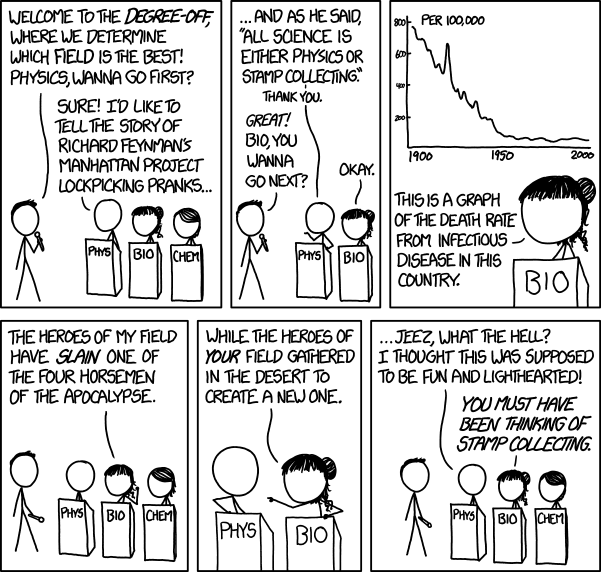
Sidenote: I’ve heard people mistakenly attribute the quote to Richard Feynman, possibly due to this comic (although I don’t think that was the intent).
What accounts for much of the progress we’ve made in fields like the biological sciences over the last 100 years? In my view, many advances stem from mathematical modeling.
Today, most scientific fields (including and especially the biological sciences) embrace the use of mathematical models and theory to describe and make predictions about the natural world. For example, and directly relevant to the comic, mathematical models were instrumental in understanding HIV viral dyanmics and recommending policies to reduce disease spread, such as during the COVID-19 epidemic.
My passion is for ecology. So, these lectures focus on mathematical tool used in ecology and evolutionary biology (although I will frequently use examples from disease ecology).
As a side note, I recently read a very interesting post suggesting that the above interpretation of the quote is entirely wrong. I’m very sympathetic to that view, but I’m trying to make a compelling point – so I won’t let this inconvenient analysis get in my way (note: this is a generally frowned upon scientific practice.)
2 Some basics of modeling a population
Keeping things general and simple, models in ecology often describe and track the population abundance of a species or multiple species (although they may keep track of many other things as well). We might write something like this:
\[ \underbrace{N(t+1)}_{\text{Abundance next time step}} = \underbrace{N(t)}_{\text{Abundance previous time step}} + \underbrace{\underbrace{B}_{\text{Total births}} - \underbrace{D}_{\text{Total deaths}}}_{\text{Within-population processes}} + \underbrace{\underbrace{I}_{\text{Total immigrants}} - \underbrace{E}_{\text{Total emigrants}}}_{\text{External population processes}} \] For example, maybe we’re interested in the population trajectory of a rabbit species over time:
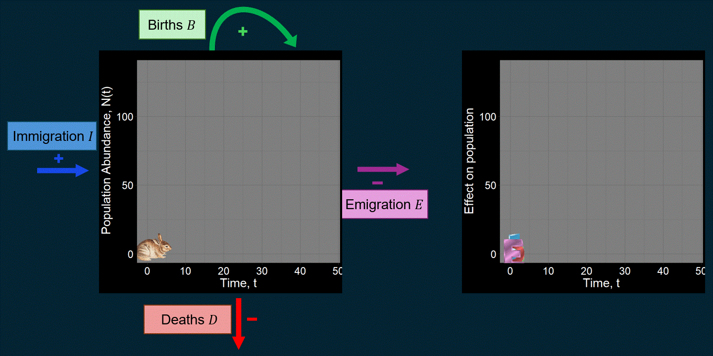
A lot of work in population ecology and community ecology is devoted to questions like: “What causes deaths?” “What affects births?” “How do and why do they vary over time?” For example, what determines \(B\) and \(D\) can be very complicated functions that could depend on anything we can imagine (the environment, \(N(t)\), predators, etc.). That is, we might think \(B = f\big(N(t)\big)\) or \(D = g(\text{Number of Predators})\), where \(f\) and \(g\) are functions that we have to come up with. You might be surprised just how many academic papers focus on changing subtle aspects of the functions used to determine \(B\) and \(D\). If we were modeling the population dynamics of a pathogen (e.g., COVID-19), \(B\) might be defined in terms of “the number of new infections” and \(D\) might be expressed in terms of the recovery rate. \(I\) might reflect infected people coming in from different cities.
The key point is that, from here, the world is our oyster and there is endless room for creativity. As a concrete example, here’s an animation that depicts the population dynamics of many tree species in a forest, based on a paper by Wiegand et al (2025):
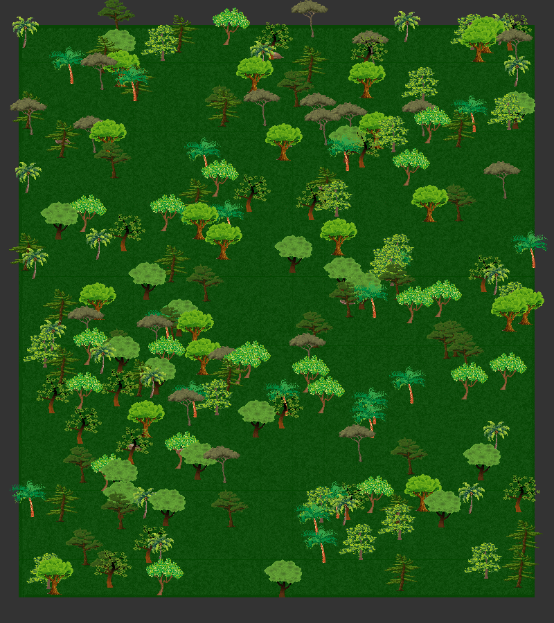
I’m personally fascinated by the insights models (such as the above) can provide into the natural world. I also simply find then fun and amusing to think about. It is my hope that you will find them entertaining and illminating as well.